Hardy-Weinberg
Equilibrium
Allele frequencies (or percentages, if you prefer) in a population
will remain in Hardy-Weinberg Equilibrium (HWE) from generation to
generation if the following assumptions are met:
- Natural selection is not occurring
- Migration (Gene Flow) is not occurring
- Mutation is not occurring
- Genetic Drift is not occurring (drift is less likely in populations of large size)
- Mating occurs at random
Although these assumptions are rarely true in the natural world,
they allow us to calculate an expected allele frequency. Significant
differences between the observed and expected frequencies indicate
that "something" (i.e. one or more of the above) is going on, and
therefore tell us that "microevolution"
is occurring.
Calculating Expected Allele and Genotype frequencies:
In the simplest possible situation we have a single gene with only two alleles. These alleles might be A and a, or A1 and A2. Let's say that A or A1= tall, and a or A2= short. Don't worry for now whether the alleles are dominant and recessive or co-dominant. They will have frequencies p and q in a population. (Because there are only two possibilities and they have to add up to 100%, p + q = 1.)
If we know the allele frequencies, we can predict the genotype frequencies. The expected genotype frequencies of the two alleles are calculated as shown. This ought to look familiar: it's
our old friend the Punnet's Square. Allele A or A1 has a frequency of p, and allele a or A2 has a frequency of q. Multiply the allele frequencies to the get the probability of each genotype.
| Allele |
|
A |
a |
| |
Frequency
|
p
|
q
|
| A |
p
|
p2
|
pq
|
| a |
q
|
pq
|
q2
|
or
| Allele |
|
A1 |
A2 |
| |
Frequency |
p
|
q
|
| A1 |
p
|
p2
|
pq
|
| A2 |
q
|
pq
|
q2
|
In other words, p2 + pq + pq + q2 = 1, or
100%. The expected frequencies of the genotypes are therefore:
|
Genotype
|
Expected Frequency
|
|
AA or
A1A1
|
p * p = p2
|
|
Aa
or A1A2
|
pq + pq (or 2pq)
|
|
aa
or A2A2
|
q * q = q2
|
Let's take a look at some graphs of this to make it a little easier to see. For values of p from 0 to 1, in intervals of 0.1, here's what we get:
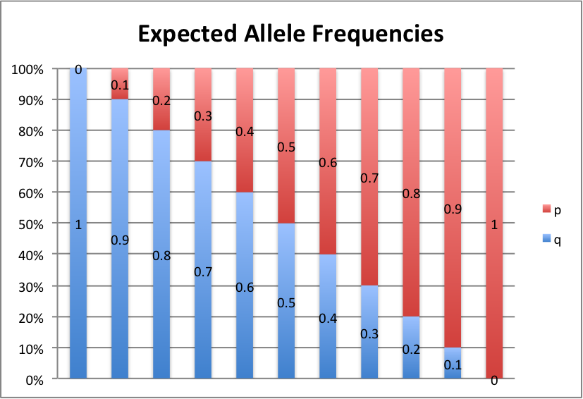
p+q=1, so p=1-q and q=1-p
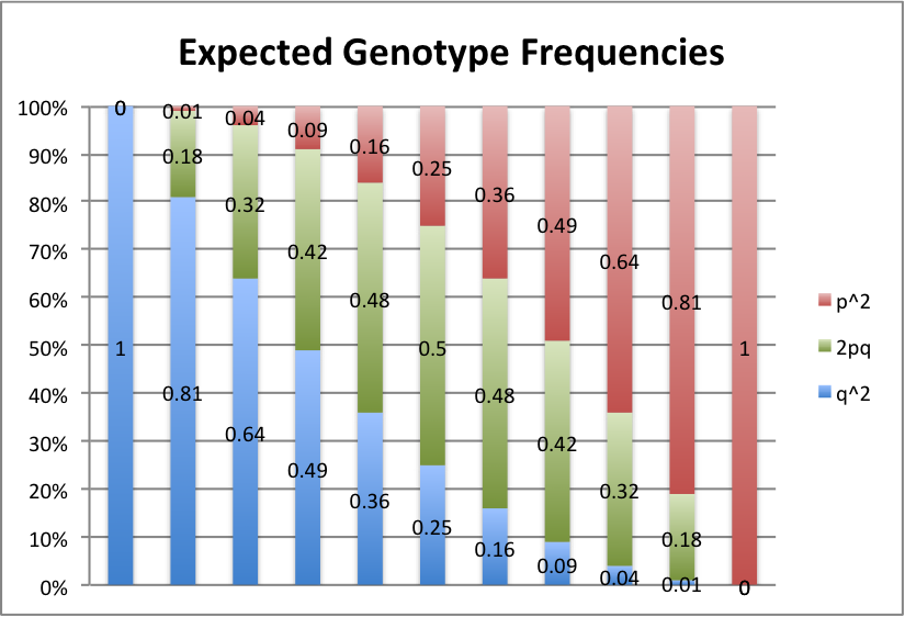
Red represents the frequency of the AA or A1A1 genotype, green is the Aa or A1A2 genotype, and blue is the aa or A2A2 genotype.
All of the above has to do with the allele and genotype frequencies we would expect to see. Next, let's look at the real world situation so we can compare.
Calculating Observed Allele and Genotype Frequencies:
In a real world population, we can only see phenotypes, not genotypes or alleles. However, in a population of genotypes AA, Aa and aa, the observed
frequency of allele A equals the sum of all of the AA genotype plus
half of Aa genotype (the A half). The observed frequency of allele a is therefore
half of the Aa individuals (the a half) plus all of aa individuals. If you know one
value, you can of course just subtract it from 1 (100%) to get the
value of the other. In other words, the observed frequency of A = 100%(AA) + 50%(Aa)
and a = 50%(Aa) and 100%(aa)
| Phenotype |
Genotype
|
Makeup |
Frequency |
| Tall |
AA
|
100% A |
p2 |
| Tall |
Aa
|
50% A and 50% a |
2pq |
| Short |
aa
|
100% a |
q2 |
or
| Phenotype |
Genotype
|
Makeup |
Frequency |
| Tall |
A1A1
|
100% A1 |
p2 |
| Medium |
A1A2
|
50% A1and 50% A2 |
2pq |
| Short |
A2A2
|
100% A2 |
q2 |
Tip: If the alleles are codominant, each phenotype is distinct (you can distinguish between tall, medium and short) and your job is easier. If the alleles are dominant and recessive, we can't visually tell the homozygous AA from the heterozygous Aa genotypes (both are tall), so it's best to start with the homozygous recessive (short) aa individuals. Count up the aa types and you have the observed q2. Then, take the square root of q2 to get q, and then subtract q from 1 to get p. Square p to get p2 and multiply 2*p*q to get the observed heterozygous Aa genotype frequency.
Conclusion:
If observed and expected genotype frequencies are
significantly different, the population is out of HWE.
| |
Genotype Frequencies |
| |
AA |
Aa |
aa
|
| Observed |
|
|
|
| Expected |
|
|
|
| Difference |
|
|
|
or
| |
Genotype Frequencies |
| |
A1A1 |
A1A2 |
A2A2
|
| Observed |
|
|
|
| Expected |
|
|
|
| Difference |
|
|
|
Question: Why might observed and expected phenotype frequencies differ? Imagine the following scenarios where natural selection is at work. Situation one favors only one tail of the distribution. Perhaps the tallest, perhaps the shortest, but not both. This is directional selection. Now imagine that both tails of the distribution are selected against, and only the middle is favored. This is called stabilizing selection. Next imagine that the extremes on both ends are favored. This is called disruptive selection. In each of these scenarios, what would happen over time?
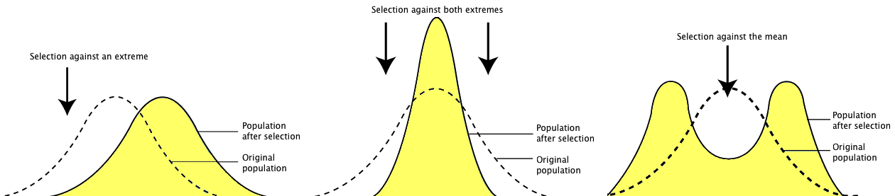
Before (dotted line) and after (yellow shaded area) directional selection, stabilizing selection, and disruptive selection.
Examples:
One common misconception is that dominant alleles will rise in
frequency and recessive alleles will decline in frequency over time.
In reality, allele frequencies will not change from one generation to
the next if the assumptions listed above are not violated. A good
example of this is human
ABO blood type. Type O blood is recessive but it remains the most
common.
In the hwe.xlsx Excel Spreadsheet, there are
three examples to help make this more concrete.
Example 1: Allele A is dominant and allele a is recessive.
Set the original frequencies of p (allele A) and q (allele a) at 0.6
and 0.4 in Generation 1. These are highlighted in blue. All other
numbers are calculated from these two original data points. The
frequency of genotype AA is determined by squaring the allele
frequency A. The frequency of genotype Aa is determined by
multiplying 2 times the frequency of A times the frequency of a. The
frequency of aa is determined by squaring a. Try changing p and q to
other values, ensuring only that p and q always equal 1. Does it make
any difference in the results?
Example 2: Alleles A1 and A2 are
co-dominant. In this case, A1 is at a frequency of 0.25
and A2 is at a frequency of 0.75.
Example 3: Alleles A and a are dominant and recessive. Note
that allele A is at very low frequency despite being dominant. Does
it increase in frequency?
Problem:
The second sometimes confusing thing about HWE is that after all
of the examples above, you may wonder if it is possible for the
observed and expected frequencies to differ. Here's an example where
they do:
In a population of snails, shell color is coded for by a single
gene. The alleles A1 and A2 are co-dominant.
The genotype A1A1 makes an orange shell. The
genotype A1A2 makes a yellow shell. The
genotype A2 A2 makes a black shell. 1% of the
snails are orange, 98% are yellow, and 1% of the snails are
black.
Observed frequency of A1 allele = 0.01 + 0.5(.98)
= 0.50 = 50%
p2 = Expected frequency of A1A1 =
0.25
2pq = Expected frequency of A1A2 = 0.50
q2 = Expected frequency of A2 A2
= 0.25
| Phenotype |
Orange |
Yellow |
Black |
|
Genotype
|
A1A1
|
A1 A2
|
A2A2
|
|
Observed
|
1%
|
98%
|
1%
|
| Expected |
25%
|
50%
|
25%
|
|
Difference
|
-24%
|
+48%
|
-24%
|
There are significantly fewer orange and black snails than expected, and significantly more yellow snails than expected. It appears that this is a case of stabilizing selection, since both tails appear to be strongly selected against.